Dimensionality Reduction (1): Principal Component Analysis

Introduction
This article explains the concept of dimensionality reduction techniques. Specifically, we introduce a method called Principal Component Analysis (PCA) to perform dimensionality reduction. In this context, dimensionality reduction does not mean selecting a subset of existing parameters but rather creating a smaller number of new parameters and expressing the data in a lower-dimensional space defined by those new parameters.
Why is dimensionality reduction necessary when analyzing data using machine learning?
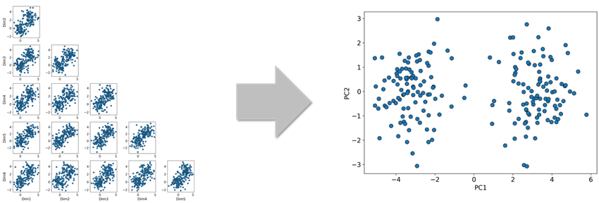
In general, handling high-dimensional data with many explanatory variables can lead to several issues. One such issue is the difficulty of gaining intuitive understanding through visualization. For example, visualizing six-dimensional data as it is can be extremely challenging. A common approach is to project the six-dimensional data onto two arbitrary parameter axes for plotting. However, this does not always allow for an intuitive grasp of the overall data distribution (see Figure 1, left).
In such cases, if the data can be reduced to two or three dimensions, it may be easier to intuitively understand the distribution within the reduced-dimensional space through visualization (see Figure 1, right). In the example shown in Figure 1, it is hard to capture the characteristics of the data when projecting the six-dimensional data onto arbitrary two dimensions. However, by applying a specific dimensionality reduction method to project the data onto two dimensions, it visually appears that the data is divided into two clusters.
This is why dimensionality reduction is often used to aid in visualization and intuitive understanding of data. The method used for dimensionality reduction in Figure 1 will be explained later in this article.
Another issue arises when the number of data points is limited relative to the number of dimensions. For example, in a high-dimensional space with 100 dimensions but only 20 data points, those points are sparsely distributed. In such a sparse setting, a machine learning model may overfit to the available data. As a result, its prediction accuracy on unseen data in the high-dimensional space may decrease.
If these high-dimensional data points can be projected into a lower-dimensional space through dimensionality reduction, and if there are enough data points to reasonably infer the distribution in that space, then the predictive accuracy in the reduced space may improve (see Figure 2). The dimensionality reduction technique used in such situations will be discussed later in this article.
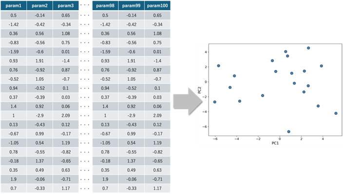
and their projection in 2D
Additionally, with high-dimensional data, the sheer number of parameters results in a significant increase in the computational resources required for processing. This leads to a considerable computational burden. By applying dimensionality reduction and converting high-dimensional data into a lower-dimensional form, it becomes possible to reduce this burden—ultimately shortening both the overall processing time and the model training time.
Principal Component Analysis
So, what kind of dimensionality reduction technique should we use to transform high-dimensional data into a lower-dimensional form?
There are many methods available for dimensionality reduction. Some of the most well-known techniques include Principal Component Analysis (PCA), Independent Component Analysis (ICA), t-Distributed Stochastic Neighbor Embedding (t-SNE), autoencoders, random projection, and kernel PCA. In this article, we will focus on Principal Component Analysis. PCA is a technique for reducing the dimensions of data by projecting it into a lower-dimensional space based on the variance of the data. To help illustrate this concept, Figure 3 below shows an example of projecting 2D data into 1D using PCA.
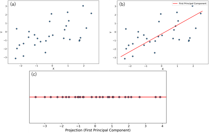
(b) Plot showing the first principal component direction (red dashed line) obtained from PCA on the 2D data;
(c) Plot of the original 2D data projected onto the principal component direction.
In Figure 3(b), the new axis indicated by the red solid line represents the direction along which the original 2D data has the greatest variance. This axis, which captures the most spread in the data, is called the first principal component. As shown in Figure 3(c), the data projected onto the first principal component exhibits more variance compared to projections onto the original x or y axes. The reason variance is used as the criterion is because greater variance typically indicates more distinguishable differences among data points, hence, more information.
Since the original data is in two dimensions, projecting it only onto the first principal component does not fully represent the original data. To address this, a second principal component is introduced, which is chosen as the direction orthogonal to the first component that has the next greatest variance. In a 2D dataset, there is only one axis orthogonal to the first principal component, so the second component is uniquely defined.
The same approach can be applied to data in higher-dimensional spaces, where we identify the first, second, third, and so on, principal components. But how far should we reduce the dimensions when projecting high-dimensional data into a lower-dimensional space? One useful concept to answer this question is the cumulative explained variance.
In PCA, principal components are chosen in the directions where the data variance is largest. The values of the original data projected onto these component directions are called principal component scores. By expressing the data through these scores, dimensionality reduction is achieved.
Explained Variance and Cumulative Explained Variance
PCA is a method that focuses on the variance in data to determine new axis directions (principal components), and reduces dimensionality by projecting the original data onto these directions. But how much should we reduce the dimensions when moving from high-dimensional to lower-dimensional space?
To answer this question, we commonly use the concept of explained variance in PCA. Explained variance refers to the proportion of the total variance in the data that each principal component accounts for. For example, if the explained variance of the first principal component is 45%, this means that the data projected onto this component captures 45% of the total variance.
During PCA, we calculate the explained variance for each principal component. We can also compute the cumulative explained variance, which is the total variance explained by the first n components added together. This cumulative value helps guide decisions such as selecting the minimum number of principal components needed to retain a desired percentage (e.g., 95%) of the original data’s variance.
Principal Component Scores and Loadings
In PCA, there are two important terms used to interpret the analysis: principal component scoresand principal component loadings. Understanding these terms is essential for making sense of PCA results.
Principal Component Score
A principal component score is defined as the value obtained by projecting the original data onto a principal component direction. When projecting a data point onto the first principal component, the score is calculated by taking the inner product (dot product) of the data point and the first principal component vector.
This resulting value is the principal component score for that data point along the first principal component axis.
For example, in a 4-dimensional space, if the first principal component vector is known, and a data point is given as (2, 3, 5, 1)ᵀ, then the score can be computed using the formula shown in Equation 1 (to follow).
\(
\begin{pmatrix}
2\\3\\5\\1
\end{pmatrix}^{ \mathrm{ T } }
\begin{pmatrix}
\frac{1}{3\sqrt{2}} \\
\frac{2}{3\sqrt{2}} \\
\frac{2}{3\sqrt{2}} \\
\frac{1}{\sqrt{2}}
\end{pmatrix}
= \frac{7}{\sqrt{2}}
\)
Equation 1: Calculation of principal component scores
Principal Component Loadings
Principal component loadings are defined as values that represent how much each axis of the original data space contributes to a principal component before dimensionality reduction. For example, suppose PCA is applied to a 10-dimensional dataset and the first principal component is obtained. In this case, each element of the first principal component vector (v_{1,1}, …, v_{1,10}) represents the degree to which each original axis contributes to the first principal component.
Standardization in PCA
In the previous explanations of PCA, we did not touch on data preprocessing. The examples discussed so far assumed that PCA was performed directly on the original data without any preprocessing. However, in many real-world data analysis cases, the original data is typically standardized before applying PCA. So, why is standardization commonly performed as a preprocessing step?
Standardization is a transformation technique used to eliminate the effects of differences in the units or scales of variables. For example, for a variable X1, we calculate its mean and standard deviation, then subtract the mean from each data point and divide the result by the standard deviation. This process standardizes the variable X1. The same procedure is applied to all other variables. As a result, each variable is transformed into a distribution with a mean of 0 and a variance of 1.
To illustrate, imagine a cube where the length is measured in centimeters, the width in millimeters, and the height in meters. If we analyze the raw numerical values directly, the actual proportions of the cube cannot be accurately represented due to the differing units. In PCA, the variance of each variable plays a crucial role. If units are not standardized, the variable measured in millimeters (e.g., the width) may appear to have the largest variance, simply due to its smaller unit scale.
However, by applying standardization, each of the variables—length, width, and height—is converted into a standardized form with mean 0 and variance 1. This equalizes the variance across all dimensions, allowing PCA to focus on the correlation between variables. Consequently, the internal structure of the data can be evaluated more accurately.
PCA in Multi-Sigma
Multi-Sigma plans to incorporate PCA as a dimensionality reduction technique for handling high-dimensional data. While Multi-Sigma currently supports up to 200 explanatory variables, applying PCA will allow the platform to process datasets with even higher dimensionality.
Moreover, even when the number of explanatory variables is 200 or fewer, using PCA can sometimes help uncover the underlying structure of the data more effectively. In Multi-Sigma, PCA will be available as a no-code feature, making it accessible to all users regardless of their technical background.
機械学習を使った分析や予測が日常的に行われる今、協調フレームとしてのMulti-Sigma®の役割は増すばかりです。
『どのような場面で活用できるのか』をもっと知りたい方や、実際の利用シーンを見てみたい方は、是非一度お気軽にご相談ください。
In a world where machine learning-based analysis and prediction are becoming everyday practices, the role of Multi-Sigma® as a collaborative framework is more crucial than ever.
If you're interested in learning more about how it can be applied or want to see real-world examples, feel free to contact us.