[Efficient Condition Exploration] Bayesian Optimization using Multi-Sigma

Have you ever experienced something like this?
“I created a sales forecast, but I have no idea how reliable it is…”
“I want to find the optimal manufacturing conditions for a product, but I can run only limited number of experiments…”

In such cases, Gaussian Process regression, and more specifically, Bayesian Optimization, which combines it with an acquisition function, can be extremely helpful.

The Importance of Understanding Prediction Reliability

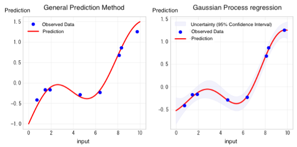
Every prediction inherently involves uncertainty. While most prediction methods only provide a single predicted value, Gaussian Process regression offers not only the predicted values but also the range of uncertainty around those predictions. Understanding uncertainty is of critical importance in both business and research & development contexts.

Grasping the uncertainty in predictions leads to more informed and strategic decision-making. For example, when predicting product quality under certain manufacturing conditions, it’s more useful to know not only that the predicted quality score is 85, but also that it is likely to fall within the range of 85 ± 3. This additional insight allows for more realistic planning. Quantitative risk assessment enables us to develop plans that account for worst-case scenarios and ensure more effective allocation of budgets and resources.

Identifying areas with high uncertainty is also crucial from a risk management perspective. It allows us to pinpoint where focused monitoring is needed and to implement preventive measures accordingly. Furthermore, by enabling objective, data-driven decision-making, it enhances the overall quality of decisions. It also makes it easier to evaluate multiple scenarios and provide more persuasive explanations.

Differences from Traditional Prediction Methods

To better understand the characteristics of Gaussian Process regression, let’s compare it with other prediction methods. Linear regression and polynomial regression typically represent data trends using straight lines or simple curves, which makes it difficult to capture complex relationships. In contrast, Gaussian Process regression can flexibly model complex, nonlinear relationships. Neural networks also offer powerful predictive capabilities, but they require large amount of data to perform effectively. Gaussian Process regression, on the other hand, works well even with relatively small datasets. This makes it especially valuable in the early stages of product development or in scenarios where collecting data is expensive or time-consuming.

Quantifying the Reliability of Predictions

In fields like product development and experimental planning, the ability to predict outcomes is critical. However, a single predicted value alone is not enough—understanding how reliable that prediction is can be just as important. Gaussian Process regression provides exactly this valuable insight by quantifying the reliability of predictions. For example, in predicting the quality of a product, the regressor can provide estimates such as: “There is a 95% probability that the quality score will fall within the range of 85±3.” Similarly, when evaluating new manufacturing conditions, it can offer uncertainty-aware insights like: “There is more than an 80% chance that the yield under these conditions will exceed 70%.”

Choosing the Right Method Based on Sample Size

When selecting a prediction method, the number of available data points is a crucial factor. Neural networks demonstrate their full potential when a large sample size is available. In contrast, Gaussian Process regression works effectively even with relatively small datasets—on the order of just a few dozen data points. This makes it especially useful in situations where evaluating prediction uncertainty is critical, or where optimizing experimental design is essential. In research and development settings where each experiment or simulation is costly, this advantage becomes particularly valuable.

Types and Characteristics of Kernels

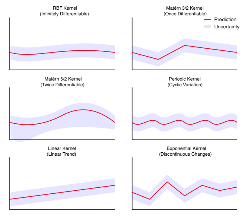
In Gaussian Process regression, one of the most important elements for capturing the characteristics of the data is the kernel. The kernel functions like a lens that helps uncover underlying features and patterns within the data. By selecting different types of kernels, it becomes possible to capture various data characteristics, such as smoothness, periodicity, and more.

• ●RBF (Radial Basis Function) Kernel

The RBF kernel, known as one of the most versatile kernels, generates infinitely differentiable smooth functions. It is well-suited for analyzing many natural phenomena, such as the relationship between temperature and reaction rate, or between pressure and deformation. When the data exhibits continuous and gradual changes, the RBF kernel delivers excellent predictive performance.

• ●Matérn 3/2 Kernel

The Matérn 3/2 kernel generates functions that are once differentiable. Compared to the RBF kernel, it allows for more abrupt changes and can handle data with a certain degree of discontinuity. It is suitable for modeling phenomena that are not perfectly smooth, such as the analysis of meteorological data or the interpolation of geospatial data.

• ●Matérn 5/2 Kernel

The Matérn 5/2 kernel generates functions that are twice differentiable, and it exhibits characteristics that are intermediate between the Matérn 3/2 and RBF kernels.
It is widely used in various applications, such as predicting material properties and optimizing production processes.

• ●Periodic Kernel

The periodic kernel is specialized for analyzing data with repeating patterns. It is well-suited for predicting data such as seasonal sales trends, periodic equipment vibration data from industrial equipment, and daily demand fluctuations. A key feature of this kernel is its ability to explicitly specify the period length.

• ●Linear Kernel

The linear kernel is suitable for data with linear trends. It is effective for predicting data that shows steady increases or decreases, such as trends in economic indicators, performance improvements due to technological advancements, and analyses of cumulative effects. This kernel is particularly well-suited for capturing long-term trends.

• ●Exponential Kernel

The exponential kernel is well-suited for capturing discontinuous changes and sudden variations in data. It is effective for modeling non-smooth phenomena such as physical phase transitions or abrupt shifts in social systems.

Role of Kernel Parameters

Each kernel has parameters designed to capture the characteristics of the data.

• ●Lengthscale

This parameter controls the characteristic length of variation in the data. Setting it to a small value allows you to capture fine-grained fluctuations in the data, while a larger value leads to smoother predictions that emphasize overall trends.

• ●Variance

Controls the overall level of variability in the predicted values. A larger value increases the uncertainty in predictions, while a smaller value decreases it (making the predictions more certain).

• ●Period

Used only in the Periodic kernel. This parameter expresses the periodicity of the data.

• ●Gaussian Noise Variance

Represents the magnitude of the noise in the observed data. If the data contain a lot of noise, set this value higher; for high-precision data, set it lower.

Gaussian Process regression in Multi-Sigma

In Multi-Sigma, users can specify the type of kernel when performing Gaussian Process regression. While it is possible to manually set the values of individual parameters, Multi-Sigma also includes an automatic parameter tuning feature. Users can build highly accurate predictive models simply by selecting the desired kernel type. Each parameter is applied based on the scale of the normalized input data.

Application to Bayesian Optimization

So far, we have explored the fundamental concepts of Gaussian Process regression and the characteristics of various kernels. Next, we will explain how this technique can be applied to optimization problems through Bayesian Optimization.

The Challenge of Efficient Optimization

In experimental and development processes, there is always a need to find the optimal conditions with a limited number of trials. Traditional optimization methods have relied either on exhaustively testing all possible conditions or on selecting conditions based on heuristics. Bayesian Optimization, on the other hand, learns from past experimental results and intelligently selects the next conditions to try. What enables this intelligent selection is the combination of prediction and uncertainty estimation provided by Gaussian Process Regression. By considering not only the predicted values but also the associated uncertainty, more efficient exploration becomes possible.

The Role of the Acquisition Function

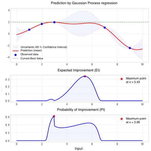
In Bayesian Optimization, acquisition functions such as Expected Improvement (EI) and Probability of Improvement (PI) serve as guiding criteria for selecting the next experimental conditions. Acquisition functions propose the most promising conditions by balancing predicted values with their associated uncertainty.

• ●Expected Improvement (EI)

The most widely used acquisition function is EI. This function quantifies how much improvement can be expected over the current best value. It identifies high potential in unexplored regions of the search space, selecting conditions that offer a promising balance between uncertainty and expected improvement. While these predictions inherently involve uncertainty, EI deliberately selects such conditions to seize opportunities for significant improvement.

• ●Probability of Improvement (PI)

When placing greater emphasis on reliable improvement, PI is a suitable choice. This function directly evaluates the probability of exceeding the current best value. It yields higher scores in regions where the prediction uncertainty is low and the predicted value is close to the current best. While substantial improvements may be less likely, this conservative approach is effective when steady performance gains are desired—such as in the optimization of mass production processes.

• ●Mean

This method considers only the mean of the prediction from Gaussian Process regression, without accounting for uncertainty. It selects the next evaluation point purely based on the highest predicted value within the search space.

Bayesian Optimization in Multi-Sigma

In Multi-Sigma, these complex processes can be executed with simple operations. By simply defining the optimization objectives and constraints, users can initiate an efficient parameter search using Bayesian Optimization. One particularly important feature is the ability to consider multiple objective functions simultaneously. For example, in materials development, it is often necessary to balance conflicting goals such as maximizing strength while minimizing cost. Multi-Sigma enables the evaluation of these trade-offs through weighted objectives, allowing users to discover practical optimal solutions. Additionally, experimental constraints can be set flexibly. Users can incorporate a variety of real-world manufacturing conditions, such as upper limits on temperature and pressure, or restrictions on raw material composition ratios.

Toward Data-Driven Decision Making

The adoption of Gaussian Process regression and Bayesian Optimization offers more than just improved efficiency—it delivers strategic value. By enabling the quantitative evaluation of prediction uncertainty, these methods support more informed and strategic decision-making. Moreover, objective judgments based on data contribute to greater transparency and accountability in decision-making processes.