Sales Prediction and Contribution Analysis Based on Retail Sales Time Series Data

This blog article focuses on an analysis using a well-known retail sales time series dataset publicly available through an online data analysis platform.

Across the retail industry as a whole – from supermarkets and department stores to home improvement centers, drugstores, apparel retailers, and convenience stores – making effective use of sales data has long been regarded as an important business priority. In particular, since the widespread adoption of POS (Point of Sale) systems, the recording and analysis of sales performance have been used extensively as a foundation for inventory management and promotional planning. In recent years, however, increasingly complex and volatile market conditions have created a growing need for more advanced analytical approaches powered by AI and machine learning.

These methods make it possible to do far more than simply summarize past sales data. They can be used to improve the accuracy of demand predictions while also helping businesses quantitatively identify the factors that are driving changes in sales. This is especially important in retail, where performance is shaped not only by internal decisions but also by a wide range of external influences, including seasonality, holidays, weather, and broader economic conditions. As a result, accurate prediction and flexible strategy development increasingly depend on comprehensive analysis that takes these factors into account.

Here, we use a publicly available retail dataset from an online data analysis platform to analyze sales patterns and contributing factors, and to consider the kinds of insights that can be drawn from them. More specifically, we look at what kinds of approaches are effective when working with sales time series data, and how those analyses can be carried out efficiently using Multi-Sigma®. We hope this will offer a practical perspective not only for people working in retail, but also for readers interested in data science.

For each department across 45 stores, the dataset includes:

• the department number
• weekly sales
• weekly date information
• an indicator showing whether the week falls on a holiday week
• the weekly average temperature in the store’s region
• regional fuel prices
• whether Discount Campaigns 1 through 5 (corresponding to Markdown 1-5 in the source data) were implemented during that week
• the consumer price index (CPI)
• the unemployment rate
• the store type (3 categories)

However, to keep the discussion clear and easy to follow, we will focus on predicting sales time series data for the first 5 departments in Store No. 1. In addition, for this analysis, the last 20 weeks of data for each department were set aside as test data, while all earlier data were used for training.

Data preprocessing (1):
Converting the date information and related variables

In the original dataset, the date information is written in a format such as “05/02/2010”. In that form, it cannot be fed directly into a machine learning model designed for numerical analysis. To address this, the date field is converted into 3 separate variables:

• Year
• Month
• Week

so that it can be used as structured numerical input. More specifically, the “Year” variable takes one of the values “2010”, “2011”, or “2012”, the “Month” variable takes a value from “1” to “12”, and the “Week” variable stores the number of weeks elapsed since the beginning of the year.

The “IsHoliday” variable indicates whether a given week is a holiday week by using the values “False” and “True.” Since these labels are not suitable for direct numerical processing, they are converted into binary values, with “False” replaced by “0” and “True” replaced by “1”.

In addition, the variables for Discount Campaigns 1 through 5 contained a large number of missing values, so all of these missing entries were filled with “0”.

Sales prediction – Part 1

After converting the data into a format suitable for numerical analysis, as described above, we built a fully connected neural network (FCNN) model using Multi-Sigma®. The model was then used to predict sales for the final 20 weeks of data in each department, and its prediction accuracy was evaluated.

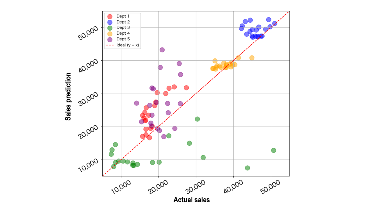
As Fig. 1 above shows, the FCNN model did not achieve strong prediction accuracy when predicting sales for the final 20 weeks in Departments 1 through 5. So why did the model perform less accurately than expected?

To explore the reasons behind this limited predictive performance, we can turn to Multi-Sigma®’s “Generating Profile” function. This is a convenient tool that automatically organizes key statistical information about the dataset – including distributions, means, and variances – simply by clicking the “Generating Profile” button on the screen. In addition, it visualizes correlations between variables at the same time, making it easier to grasp the relationships among features at a glance.

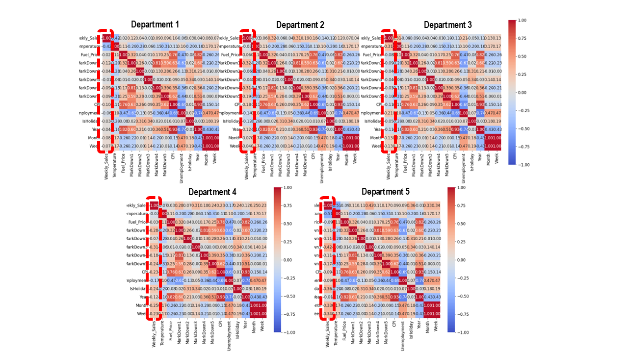
Here, the correlations within the data for each department are summarized in Fig. 2 below. The most important area to focus on is the region outlined by the red dotted line. This section shows the correlations between weekly sales and each input variable. As can be seen, there are very few variables that exhibit a clear correlation with sales. Of course, this does not mean that having just one strongly correlated variable would automatically be enough. At the very least, however, it suggests that the current set of variables may not provide enough information to build a highly accurate machine learning model.

Data preprocessing (2):
Variable transformation and feature expansion

When working with time series data, there are many possible analytical approaches. In a case like this, where an FCNN is used, one of the key questions is how past information should be incorporated into the model. This is important because an FCNN is not especially well suited, by design, to learning the “flow” or “trend” of time series data on its own. For that reason, explicitly feeding the model information about past sales and surrounding conditions can, in some cases, lead to better predictive performance.

With that in mind, the following variables were added in this analysis:

• Sales data from 1 to 4 weeks earlier, along with their total value:
  →  This was done to capture how recent sales levels may be affecting current sales behavior.
• Discount Campaigns 1 through 5 from the previous week, along with their total value:
  →  This was added to examine how the timing of discount campaigns may influence sales in the following week.
• The previous week’s unemployment rate, CPI, and whether the previous week was a holiday week or not:
  → These variables were included to take into account the possible effects of macroeconomic indicators and calendar-related events on sales.

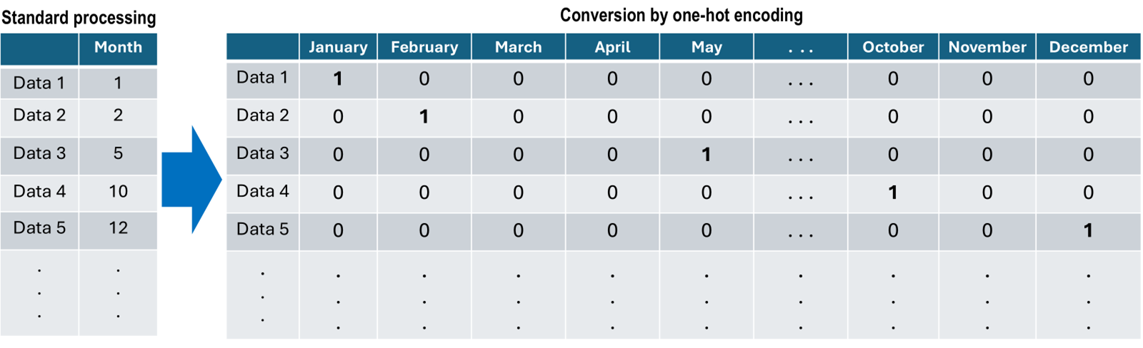
Categorical variables such as “Year” and “Month” were also converted into numerical form using one-hot encoding, represented by “0” and “1”, so that the model would not interpret them incorrectly. One-hot encoding is a common method used in machine learning when categorical data such as “month” cannot simply be entered as raw numbers. If such values are used directly, the model may mistakenly assume that the numbers carry an inherent order/size relationship, or continuity/sequence. One-hot encoding avoids this by creating a separate column (variable) for each category and representing whether that category applies using either “0” or “1”.

As a result, the model can learn the presence of each category correctly without imposing a false numerical relationship between them. This is particularly useful in cases where, for example, “March, May, and July” have a positive effect on sales, while “January, February, and October” have a negative effect. If the model were given only a single variable called “Month”, it would have difficulty capturing those kinds of irregular relationships appropriately. One-hot encoding helps solve exactly that problem.

In addition, the number of weeks elapsed since the beginning of the year was transformed using sine and cosine functions so that the model could better capture time-based seasonality, in other words, the fact that patterns repeat on a yearly cycle. This helps the model understand more naturally that, for example, “Week 52 at the end of the year” and “Week 1 at the beginning of the next year” are actually adjacent points in time.

One of the most important things to watch out for when designing features like these is information leakage. This happens when a model unintentionally uses future information during training – information that would not actually be available at the time of prediction. When that happens, the model may appear to perform extremely well on training data, yet prove far less useful in real prediction situations.

A particularly common source of this problem lies in how validation data are split. In many standard machine learning workflows, including those using general models such as FCNNs, training and validation data are often divided randomly. However, if this kind of random split is applied to time series data, future information can easily leak into the training phase, which is one of the most typical causes of information leakage.

For example, if a record containing sales data from October 2012 is included in the training data, while the immediately preceding September data are included in the validation data, the model is effectively making predictions while “looking into the future”. This is far removed from any real operational scenario and significantly undermines the reliability of model evaluation.

To address this issue, Multi-Sigma® has a function that allows the validation set to be split so that it contains only future data relative to the training set. By using this function, it becomes possible to avoid models that perform with high accuracy during training but then suffer a major drop in accuracy in actual prediction situations. As a result, more reliable prediction can be achieved even in real-world use.

Sales prediction – Part 2

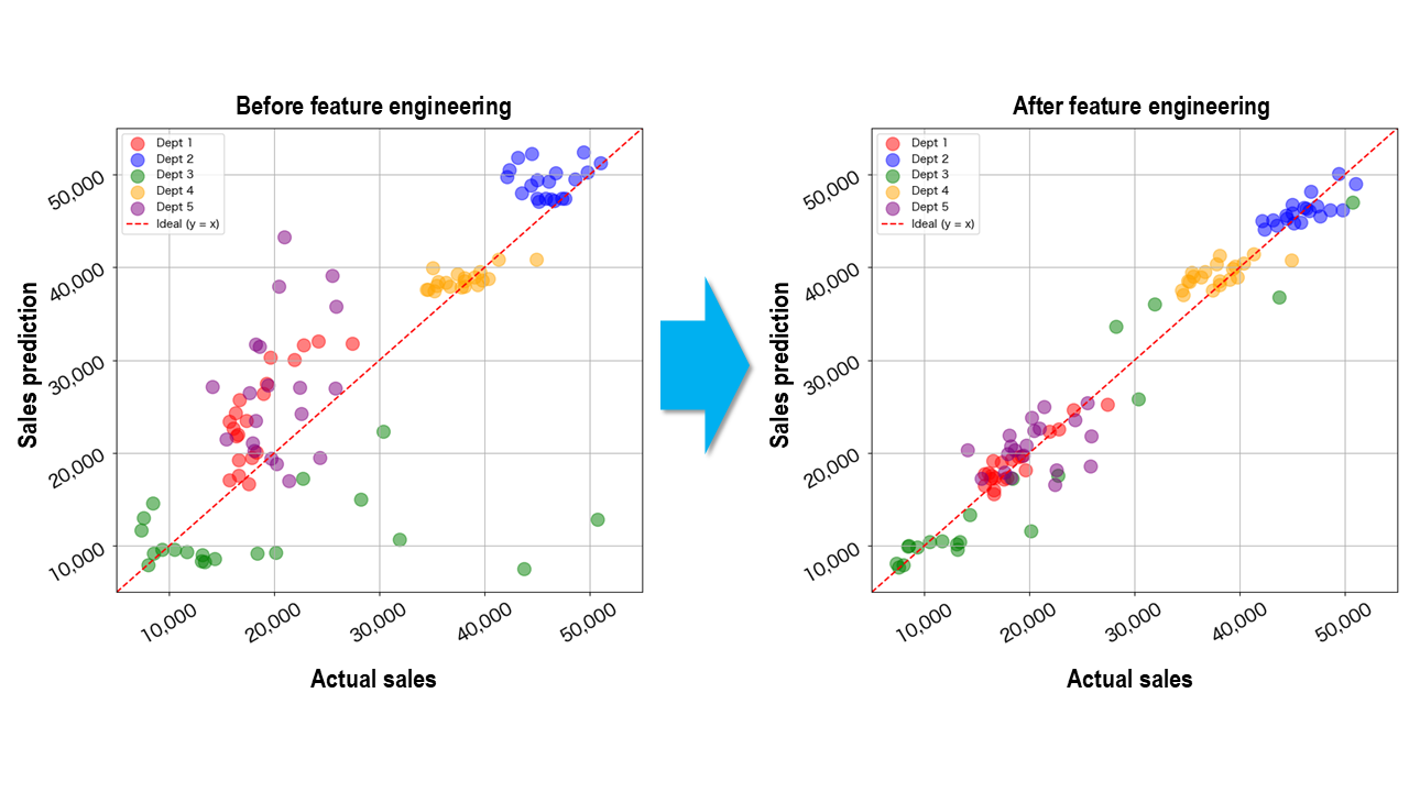
By combining the feature engineering described above with Multi-Sigma®’s Validation function designed to prevent information leakage, the accuracy of sales prediction improved substantially across all departments. This improvement can be seen by comparing the initial prediction results shown in Fig. 4 (left) with the updated results (right).

Under the earlier approach, there was a possibility that future information had been mixed into the validation data during training, creating a risk that the model’s apparent performance would diverge from its actual prediction accuracy. In the present approach, however, that risk was avoided. At the same time, the feature engineering helped the model learn the real structure of the time series data more appropriately. As a result, it became possible to achieve predictions that are not only more accurate, but also more reliable in real-world use.

Marketing strategies based on sales data

What machine learning models do best is make predictions for unseen data. Even so, prediction with time series data is never straightforward and usually requires a good deal of careful design. There is also another challenge: with machine learning models such as FCNNs, even when prediction accuracy is high, it can still be difficult to interpret why the model arrived at a particular result. In other words, even if future sales can be predicted with high accuracy, that does not automatically make it easy to understand what is actually driving those changes in sales.

This is where the Contribution Analysis function built into Multi-Sigma® becomes especially useful. By using it, the variables that influenced sales can be visualized and analyzed more clearly. That, in turn, makes it possible to draw practical marketing insights such as the following:

• which discount campaigns were associated with improved sales
• how external factors such as seasonality and holidays were associated with sales
• how past sales trends continue to influence current sales

In this way, the analysis does not stop at prediction alone. One of the major strengths of using Multi-Sigma® is that it also helps reveal why sales may have increased or decreased.

As a result, it becomes possible to go beyond numerical prediction and gain insights that can support more strategic decision-making.

What sales data reveal about the effectiveness of discount campaigns

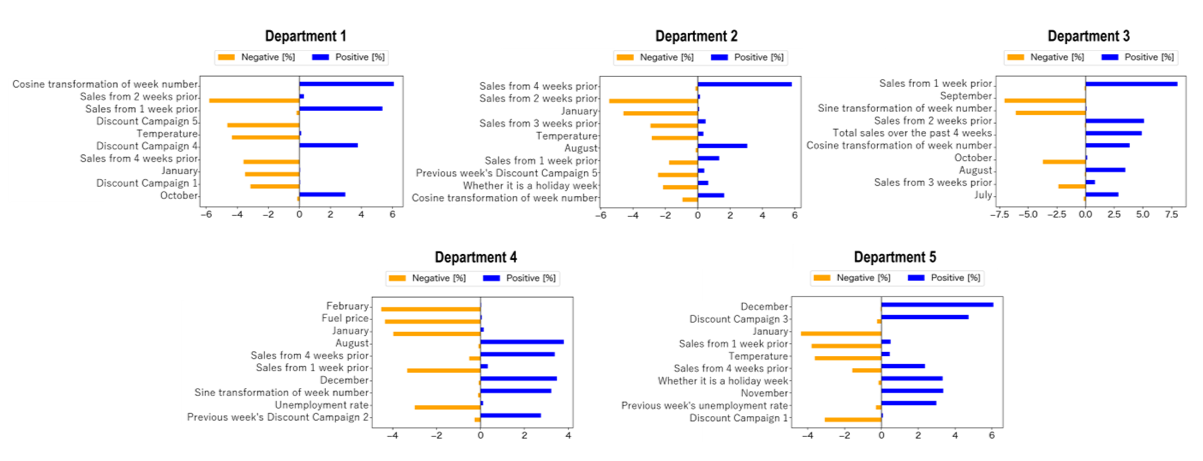
Fig. 5 below shows the results of the Contribution Analysis for each sales department. These results suggest that, in some departments, discount campaigns implemented during the current week and the previous week were associated with sales performance.

Department 1, for example, showed a particularly interesting pattern. When Discount Campaign 4 was implemented, sales tended to improve, whereas Campaigns 1 and 5 were associated with weaker sales. The exact reason is not clear from the available data, but one possible explanation is that Campaigns 1 and 5 may have been aimed at other departments. If that was the case, customers may simply have spent more of their budget there, leaving less to spend in Department 1.

A similar point can be seen in Department 4, where Discount Campaign 2 implemented in the previous week was associated with higher sales. Here again, several possible interpretations can be considered. For example, if Campaign 2 involved products that are consumed quickly, such as groceries or daily necessities, purchases made during the previous week may have encouraged repeat purchases the following week. Another possibility is that the previous week’s Campaign 2 was functioning as a proxy variable, meaning that some other factor may in fact have been influencing sales.

As this shows, it is difficult to draw firm conclusions when the publicly available variables are limited. Even so, the model output does reveal patterns that suggest a relationship between these campaigns and sales performance. Similar signs can also be seen in other departments, where Discount Campaigns appear to have influenced sales in one way or another.

This is where the Contribution Analysis becomes especially valuable. It can provide practical insights into questions such as: which campaigns are effective for which departments, and when their effects are most likely to appear. That kind of insight can become a powerful asset when planning marketing strategy.

Promotional strategies based on holidays, sales trends, and event-driven fluctuations

Similarly, Fig. 5 also suggests that, in some sales departments, factors such as seasonality and holidays influence sales.

Department 5 offers a particularly clear example. Sales show a marked upward trend from November through December, and an additional increase can also be seen during holiday weeks. Taken together, these patterns suggest that Department 5 may handle a large number of products that perform especially well during the end of the year shopping season, such as the Christmas period. By contrast, sales appear to fall sharply once January begins, which suggests a pattern in which demand peaks at the end of the year and is then followed by a post-holiday decline.

Another notable point is that, in this department, sales tended to decrease during weeks when Discount Campaign 1 was implemented. If that campaign was being run during periods such as November or December, when sales would normally be expected to grow, it may indicate that the campaign strategy itself was not delivering the effect that had been intended. Looking closely at patterns like these can help companies evaluate the likely relationship between their campaigns and sales outcomes and refine the timing of future actions.

In practical marketing analysis, this kind of insight is extremely valuable. It helps businesses reassess, based on detailed data, which campaigns should be carried out, in which departments, and at what times of year.

One particularly interesting finding in the analysis was the cyclical pattern seen in Department 3 sales. In this department, the sine function applied to the number of weeks from the beginning of the year had a negative effect, while the cosine-transformed variable had a positive effect, suggesting that sales tend to rise and fall in a regular cycle over time.

The results of the Contribution Analysis also show a clear seasonal pattern: sales tend to increase from July to August, then decline from September to October.

Another important finding was that recent sales trends in this department were useful for predicting future sales. More specifically, when sales were high one or two weeks earlier, that upward trend often continued into the current week as well. On the other hand, when sales had been high three weeks earlier, current-week sales tended to decline somewhat. This suggests that the sales trends in this department tend to persist for only about two to three weeks.

Understanding patterns like these can lead directly to practical action. For example, campaigns can be timed to coincide with periods when sales are more likely to rise, while inventory can be adjusted more effectively to reduce the risk of running out of stock. In addition, during periods when sales tend to weaken, businesses can respond more strategically by introducing new products or strengthening cross-selling efforts.

Marketing strategy informed by external factors and sales data

Furthermore, Fig. 5 also shows that, in some sales departments, external factors such as the unemployment rate and fuel prices appear to be influencing sales.

Department 4 provides a clear example of this pattern. Sales tended to decline when unemployment and fuel prices rose, which may reflect pressure on consumers’ disposable income as well as reduced mobility. Sales also appeared to weaken during colder months such as January and February, suggesting that seasonal conditions may be playing a role as well. This naturally raises an important question: for departments that are especially sensitive to external factors, what kind of marketing strategy is likely to be effective?

To begin with, during periods of rising fuel prices or increasing unemployment, customers may visit stores less frequently. In that kind of environment, one possible response is to focus on raising basket size at the time of purchase – for example, by promoting bundle offers that encourage larger purchases or by strengthening pathways to online purchasing through e-commerce channels. In addition, if the products handled by those departments are not everyday necessities, another reasonable strategy may be to avoid pushing sales too aggressively and instead place greater emphasis on other departments where demand is more stable, thereby helping maintain overall store performance.

The key point here is that these external factors themselves are not something the retailer can control. Precisely for that reason, it becomes important to treat them as “predefined constraints”, understand how they are affecting sales, and then respond with flexible, adaptive marketing measures.

Conclusion

In this blog article, we worked with publicly available retail data, carried out some basic preprocessing, and used Multi-Sigma® to perform sales prediction and Contribution Analysis. In particular, we introduced an analysis workflow that can also be applied in practice – from feature design for time series data, to validation methods for preventing information leakage, to the visualization of the factors behind sales performance, including promotions, seasonality, and external factors.

In real marketing analysis and day-to-day business use, there are also several more advanced perspectives worth considering, such as:

• evaluating the combined effect of holidays and discount campaigns
• gaining a broader optimization perspective by aggregating and comparing sales fluctuations across departments
• examining the medium/long-term impact of discount campaigns and promotions (including lag effects, repeat purchase behavior, etc.)

Although we could not cover them fully in this blog, Multi-Sigma® also includes more advanced tools designed to support strategic decision-making, such as its “Optimization function” and “Chain Analysis function”. For example, it can be used to propose the most suitable combination of measures for achieving a specific sales target, or to capture interactions across multiple departments and multiple promotional actions. Functions like these can be especially powerful when decisions need to be made in complex real-world settings.

Multi-Sigma® is often used in research and development settings, but it can also be applied very effectively in sales analysis and marketing when used in ways that match the objective at hand. In that sense, it offers a practical way to combine quantitative decision-making with actual business practice. Looking ahead, future data utilization will likely depend not only on prediction but also on understanding and optimization, which will be key to strengthening a company’s competitiveness.

（Data source）
https://www.kaggle.com/datasets/manjeetsingh/retaildataset